A brief digression into Probability & Statistics
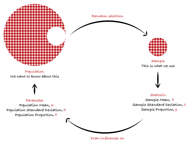
We measure the sample using statistics in order to draw inferences about the population and its parameters. Samples are collected through random selection from a population. This process is called sampling.
Types of statistics:
- Descriptive: Number that describes or gives a gist of the population data under consideration.
- Inferential: Making conclusion about the population. Notion of variability: Degree to which data points are different from each other or the degree to which they vary.
Methods of sampling data:
- Random sampling: Every member and set of members has an equal chance of being included in the sample.
- Stratified random sampling: The population is first split into groups. The overall sample consists of some members from every group. The members from each group are chosen randomly. Most widely used sampling technique.
- Cluster random sample: The population is first split into groups. The overall sample consists of every member from some groups. The groups are selected at random.
- Systematic random sample: Members of the population are put in some order. A starting point is selected at random and every nth member is selected to be in the sample.
Types of Statistical Studies:
- Sample study(informal term): Taking random samples to generate a statistic to estimate the population parameter.
- Observational study: Observing a correlation but not sure of the causality.
- Controlled experiment: Experimenting to confirm the observation by forming a control group and treatment group. It is done by randomly assigning people or things to groups. One group receives a treatment and the other group doesn’t.
Running an experiment is the best way to conduct a statistical study. The purpose of a sample study is to estimate certain population parameter while observational study and experiment is to compare two population parameters.
Describing data Central Tendency: There are different ways of understanding central tendency Mean: Arithmetic mean value Median: Middle value Mode: Highest frequency value e.g. Samples of observations of a variable
\(x_i\) = 2, 4, 7, 11, 16.5, 16.5, 19
\(n\) = 7
Mean \(\bar{x} = \sum_{i=1}^n \frac{x_i}{n}\) = (2 + 4 + 7 + 11 + 15 + 16.5 + 19)/7 = 10.643
Median = 11
Mode = 16.5
Median is preferred when the data is skewed or subject to outliers.
WARNING: A median value significantly larger than the mean value should be investigated!
Measuring spread of data:
Range: Maximum value – Minimum value = 19 – 2 = 17
Variance: \(s_{n-1}^2 = \sum_{i=1}^n\frac{\left({x_i} – \bar{x}\right)^2}{n-1}\)
Standard Deviation: \(s_{n-1} = \sqrt{Variance}\)
Range is a quick way to get an idea of the spread.
IQR takes longer to compute but it sometimes gives more useful insights like outliers or bad data points etc.
Interquartile Range: IQR is amount of spread in the middle 50% of the data set. In the previous e.g.
Q1(25% of data) = (2 + 4 + 7 + 11)/4 = 6
Q2(50% of data) = 11
Q3(75% of data) = (11 + 16.5 + 16.5 + 19)/4 = 15.75
IQR = Q3 – Q1 = 15.75 – 6 = 9.75
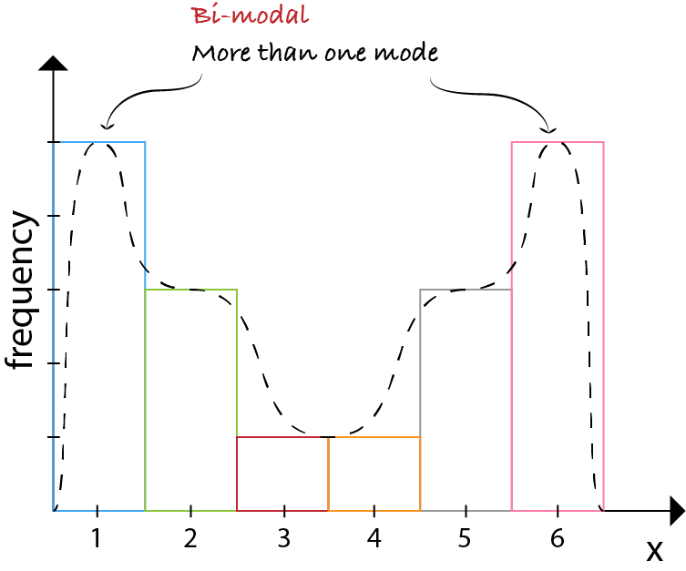
Questioning the underlying reason for distributional non-unimodality frequently leads to greater insight and improved deterministic modeling of the phenomenon under study.
- Very common in real-world data.
- Best practice is to look into this.
Plotting Data
- Bar chart: It is made up of columns plotted on a graph and used for categorical variable.
- Frequency histogram(Histogram): It is made up of columns plotted on a graph and used for quantitative variable. Usually obtained by splitting the range of a continuous variable into equal sized bins(classes).
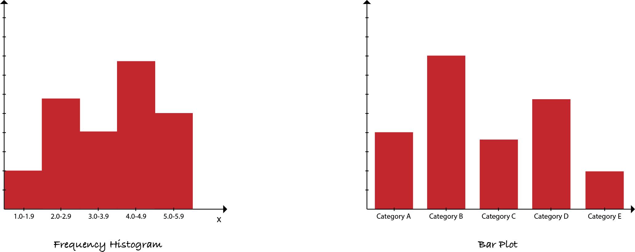
Both display relative frequencies of different variables. With bar charts, the labels on the X axis are categorical; with histograms, the labels are quantitative. Both are useful in detecting outliers(odd data points).
- Boxplots: The boxplot (a.k.a. box and whisker diagram) is a standardized way of displaying the distribution of data based on the five number summary: minimum, first quartile, median, third quartile, and maximum. In the simplest boxplot the central rectangle spans the first quartile to the third quartile (the interquartile range or IQR). A segment inside the rectangle shows the median and “whiskers” above and below the box show the locations of the minimum and maximum. The extreme values (within 1.5 times the interquartile range from the upper or lower quartile) are the ends of the lines extending from the IQR. Points at a greater distance from the median than 1.5 times the IQR are plotted individually as asterisks. These points represent potential outliers.

Shape
- Skewness: Measure of degree of asymmetry of a variable.

-
Skewness = \(\frac{1}{N}\sum_{i=1}^{N}\frac{(x_i-\overline{x})^3}{\sigma^3}\)
- Value of 0 indicates a perfectly symmetric variable.
- Positive skewness: The majority of observations are to the left of the mean.
- Negative skewness: The majority of observations are to the right of the mean.
- Kurtosis: A measure of how “tailed” a variable is.
- Variables with a pronounced peak near the mean have high kurtosis.
- Variables with a flat peak have a low kurtosis.
-
Kurtosis = \(\frac{1}{N}\sum_{i=1}^{N}\frac{(x_i-\overline{x})^4}{\sigma^4}\)
- Values for skewness and kurtosis near zero indicate the variable approximates a normal distribution.
Sample Statistic and Population Parameter
Each sample statistic has a corresponding unknown population value called a parameter. e.g. population mean, variance etc. are called parameter whereas sample mean, variance etc. are called statistic.
| Sample Statistic | Population Parameter | |
|---|---|---|
| Mean | \(\bar{x}=\sum_{i=1}^n\frac{x_i}{n}\) | \(\mu=\sum_{i=1}^N\frac{x_i}{N}\) |
| Variance | \(s_{n-1}^2=\sum_{i=1}^n\frac{({x_i-\bar{x}})^2}{n-1}\) | \(\sigma^2=\sum_{i=1}^N\frac{({x_i-\mu})^2}{N}\) |
| Standard Deviation | \(s\) or \(s_{n-1}\) | \(\sigma\) |
There are many more sample statistics and their corresponding population parameters.
Probability
Probability: The likelihood of an event occurring.
Probability of an event = \(\frac{\text{# of favourable outcomes}}{\text{Total # of possible outcomes}}\)
Conditional Probability: The probability of an event occurring given that another event has occurred.
Conditional Probability of an event \(P\left(A\vert{B}\right) = \frac{P\left(A\cap{B}\right)}{P\left(B\right)} \implies\) A is dependent on B
Bayes Theorem: \(P\left(A\vert{B}\right) = \frac{P\left(B\vert{A}\right)P\left(A\right)}{P\left(B\right)}\)
Probability Distribution:
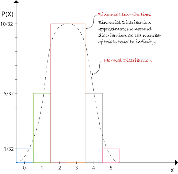
A mathematical function that, stated in simple terms, can be thought of as providing the probability of occurrence of different possible outcomes in an experiment. Let’s say we have a random variable 𝑋 = # of HEADS from flipping a coin 5 times.
Central Limit Theorem
Suppose that a sample is obtained containing a large number of observations, each observation being randomly generated in a way that does not depend on the values of other observations and arithmetic average of the observations is computed. If this procedure of random sampling and computing the average of observations is performed many times, the central limit theorem says that the computed values of the average will be distributed according to the normal distribution (commonly known as a “bell curve”). A simple example of this is that if one flips a coin many times the probability of getting a given number of heads in a series of flips should follow a normal curve, with mean equal to half the total number of flips in each series as shown previously.
Sampling distribution of the sample mean
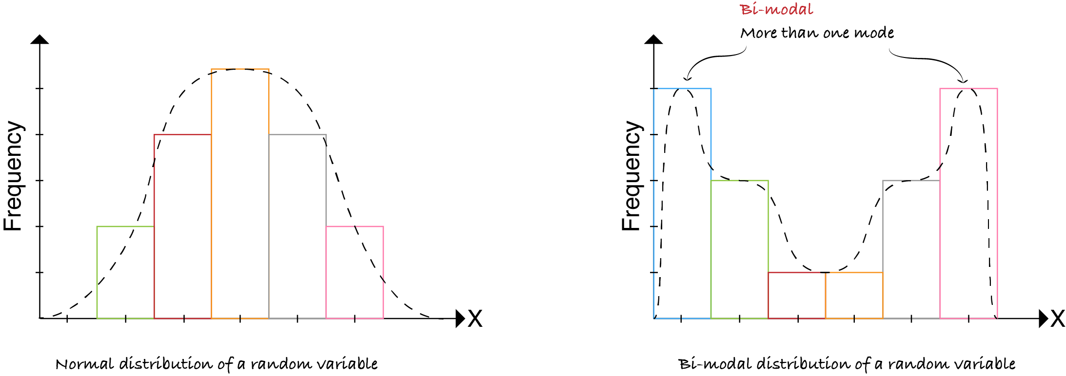
Random variables can have different distribution patterns. They can be normal or multi-modal as shown below.
To plot a sampling distribution of sample means(can be mode, median etc.) we draw samples of certain size(say 3) from a distribution and compute its mean.
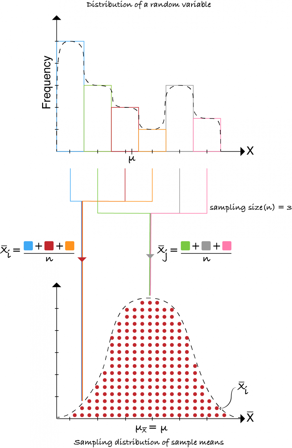
Note: The mean of sampling distribution(mean of means) is same as the population mean \((\mu_{x} = \mu)\). As the number of samples \((S_{i})\) approach infinity the curve approximates a normal distribution.
Standard Error
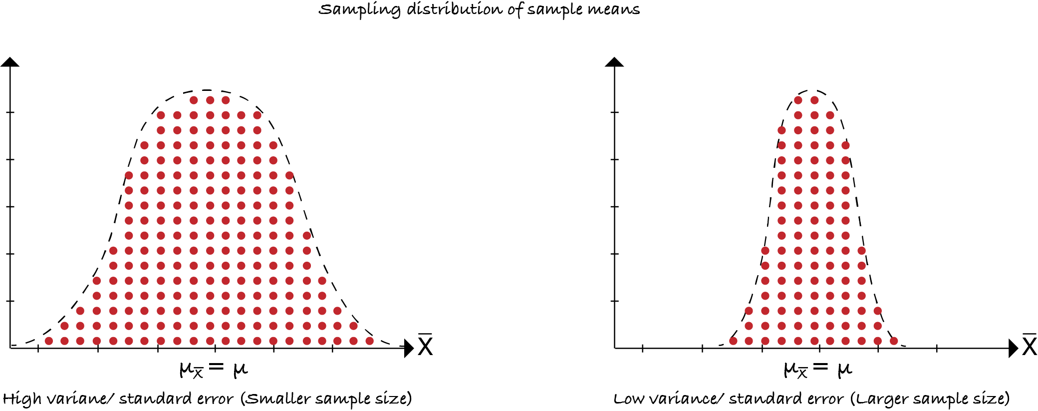
Variance of the sampling distribution of the sample mean. The standard error of the mean is the expected value(average) of the standard deviation of several samples, this is estimated from a single sample as:
\(SE_{\bar{x}}^2\) \(=\) \({s^2}\over{n}\) \(\implies\) larger the sample size lower the variance. \(s\) is standard deviation of the sample, \(n\) is the sample size.
WARNING:
\(SE_{\bar{x}}\) = sampling distribution standard deviation (not sample standard deviation).
Confidence Interval
- Each sample statistic has a corresponding unknown population value called parameter.
- How well these sample statistic estimate the underlying population value?
- Confidence interval is the range which is likely to contain the population parameter of interest.
- Confidence intervals can be 1 sided or 2 sided. We choose the type of confidence interval based on the type of test we want to perform.
- Confidence interval(2-sided, let’s say has 95% confidence level) can be interpreted as if the same population is sampled on numerous occasions, the resulting intervals would contain the true population parameter 95% of the time.
- We can only guess the range that our estimated parameter falls in and not about its exact value.
- 3 \(\sigma\) or 68-95-99.7 rule: The 68–95–99.7 rule is a shorthand used to remember the percentage of values that lie within a band around the mean in a normal distribution with a width of two, four and six standard deviations, respectively. In mathematical notation, these facts can be expressed as follows, where \(X\) is an observation from a normally distributed random variable, \(\sigma\) is the mean of the distribution, and \(\sigma\) is its standard deviation:
𝑃(𝜇 − 𝜎 ≤ 𝑋 ≤ 𝜇 + 𝜎) ≈ 0.6827
𝑃(𝜇 − 2𝜎 ≤ 𝑋 ≤ 𝜇 + 2𝜎) ≈ 0.9545
𝑃(𝜇 − 3𝜎 ≤ 𝑋 ≤ 𝜇 + 3𝜎) ≈ 0.9973
- Significance level or 𝛼 level: The alpha level is the probability/ percentage of values that lie outside the confidence interval.
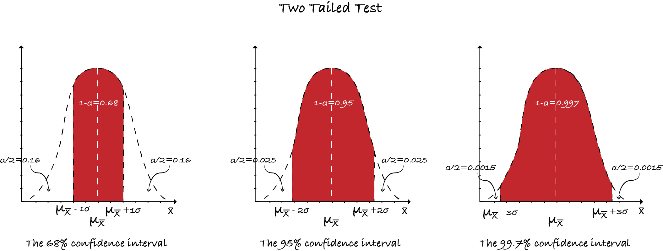
- Confidence level or 1-𝛼 level: The confidence level is the probability/ percentage of values that lie inside the confidence interval.
NOTE: In case of two tailed test, area under the curve(AUC) of the sampling distribution curve gives the probability of finding a specific value of statistic (𝑋) in a particular interval (𝜇 – 𝑛𝜎, 𝜇 + 𝑛𝜎), 𝑛 ∈ 𝐑. Therefore as the confidence level increases accuracy of the estimated parameter goes down. We usually do a two tailed test. For details on one-two tailed tests: One-Two tailed tests
How to compute a confidence interval (when population std. deviation is known and sample size is larger than ~30) Compute the standard error of the sampling distribution \({\sigma}\over{\sqrt{n}}\). Choose the desired confidence level and its corresponding significance level or alpha value. Determine the value of \(z_{\alpha \over {2}}\) (for two sided confidence interval) also called the 𝑧-score. Compute the confidence interval \(\bar{x}{\pm}{z_{\alpha/2}}\frac{\sigma}{\sqrt{n}}\)
NOTE: 𝑧-score or 𝑠𝑡𝑎𝑛𝑑𝑎𝑟𝑑-score = (𝑥−𝜇)/𝜎 ⇒ Number of standard deviations away 𝑥 is from its mean.
𝛼 = 1 – 𝑐𝑜𝑛𝑓𝑖𝑑𝑒𝑛𝑐𝑒 𝑙𝑒𝑣𝑒𝑙 / 100. We use 𝛼 for one sided test and 𝛼/2 for two sided test to compute the z-score.
𝛼 = 𝑠𝑖𝑔𝑛𝑖𝑓𝑖𝑐𝑎𝑛𝑐𝑒 level = 𝑡𝑦𝑝𝑒 𝐼 error rate
Hypothesis A statistical hypothesis, sometimes called confirmatory data analysis, is a hypothesis that is testable on the basis of observing a process that is modeled via a set of random variables.
Hypothesis Testing A formal process to determine whether to accept or reject the null hypothesis based on statistical inference.
- Null hypothesis: What would be expected if there was nothing unusual about the data. Can be thought of as the absence of effect or generally accepted wisdom.
- Alternative hypothesis: Opposite of the null hypothesis. Can be one tailed or two tailed hypothesis test.
- There are five steps in hypothesis testing:
- Making assumptions
- Stating the research, null and alternate hypotheses and selecting (setting) alpha
- Selecting the sampling distribution and specifying the test statistic
- Computing the test statistic
- Making a decision and interpreting the results
We will discuss these test statistics in detail as we go along.
Type I & Type II errors
- Type 1 Error: The type I error rate or significance level is the probability of rejecting the null hypothesis given that it is true. It is denoted by the Greek letter 𝛼 (alpha) and is also called the alpha level. Often, the significance level is set to 0.05 (5%), implying that it is acceptable to have a 5% probability of incorrectly rejecting the null hypothesis.
- Type 2 Error: When one fails to reject the null hypothesis when in reality it should be rejected.
| Table of error types | Null hypothesis $$(H_0)$$ | ||
|---|---|---|---|
| True | False | ||
| Decision About Null hypothesis $$(H_0)$$ | Reject | Type I error (False Positive) | Correct inference (True Positive) |
| Fail to reject | Correct inference (True Negative) | Type II error (False Negative) | |
NOTE: “failing to reject the null hypothesis” is NOT the same as “accepting the null hypothesis”. It simply means that the data are not sufficiently persuasive for us to prefer the alternative hypothesis over the null hypothesis. Always take the conclusions with a grain of salt.
Problem Assume we sample 10 (n=10) widgets and measure their thickness. The mean thickness of the widgets sampled is 7.55 units \((\bar{x}=7.55)\) with a standard deviation of 0.1027 (s=0.1027). But we want to have widgets that are 7.5 units thick. Compute the confidence interval for the mean for a given level of Type I error (significance or alpha level or probability of incorrectly rejecting the null hypothesis).
Solution Let’s assume that 𝛼 = 0.05 or 5%
- Null hypothesis: Mean thickness = 7.5 units
- Alternate hypothesis: Mean thickness ≠ 7.5 units(two sided test)
- Compute the confidence interval for a given level of Type I error or alpha level.
- If the test statistic (\(\bar{x}\)) falls within the confidence interval, the null hypothesis is rejected else it is accepted in favor of the alternative hypothesis.
NOTE: Since the sample size is small and the population std. deviation is unknown we can’t use normal distribution z-score to compute the confidence interval. Instead we will use t-distribution t-score discussed further to compute confidence interval. The statistic may be different but the approach to compute confidence interval is still the same. For details on confidence interval and how to compute it: Confidence interval.
Enjoy Reading This Article?
Here are some more articles you might like to read next: